In a world increasingly driven by artificial intelligence (AI), understanding the reasoning behind AI-based algorithmic decisions has become paramount. Enter Shapley values, or SHAP -–(SHapley Additive exPlanations) for short - a mathematical concept that has emerged as a powerful tool for shedding light on the inner workings of complex algorithmic systems.

From the genius of Harvard and Princeton trained mathematician and Nobel Prize Laureate Lloyd Shapley, Shapley values are one of the most widely used methods for interpreting the output of AI and machine learning (ML) models. A game theorist at heart, Shapley originally developed his eponymous concept in the realm of cooperative game theory. In that context, Shapley values are used to determine how much each player contributes to a collective payoff. Yet, SHAP’s potential and impact transcended its original, economic origins to become essential for unraveling the behavior and intricacies of AI and ML models.

Shapley values have found a new application in the burgeoning field of AI. By treating the features (predictors or predictor variables) of a model as "players" in a cooperative game, we can quantify their individual contributions to a specific prediction made by the model. This breakthrough has unlocked exciting possibilities for making AI and ML models more transparent, accountable and trustworthy.

Delving into the formula for Shapley values can uncover their potential and explore how they can transform our understanding of sophisticated AI and ML models.

According to Lloyd Shapley’s formula, the Shapley value, or the overall contribution, to a model’s prediction, assigned to a predictor variable of interest is calculated as follows:

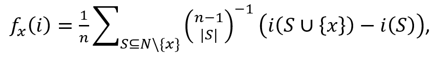
whereas:

• x is the variable of interest,
• i is a specific data point in the dataset, 
• n is the number of predictors in the model being evaluated, 
• N designates the set of the n predictor variables,
• S is a s subset of predictors from N,
• iS is the prediction from a model with predictors only from S,
• iS∪x is the prediction from a model containing x and the predictors from S,
• and the summation is applied over all possible combinations S of N that do not contain the variable of interest.

We can visualize the workings of this formula with the following simple example. Suppose we have built a predictive model with only three predictor variables X₁, X₂, and X₃, and we are interested in the overall contribution of X₂ to this model’s prediction for a specific data point. The model itself could be a form of regression or some more advanced black box model, such as a neural network or support vector machine. For simplicity’s sake, we will ignore variable interactions. Including the null set (a model with no predictors), there are 2³ = 8 possible combinations of predictors, i.e. in our example, n = 3 and S = 8. The diagram below represents these eight possible models, arranged in levels according to the number of variables they contain. In addition to the variable combinations, in each cell I have also included the model prediction for the data point that each respective variable combination produces.

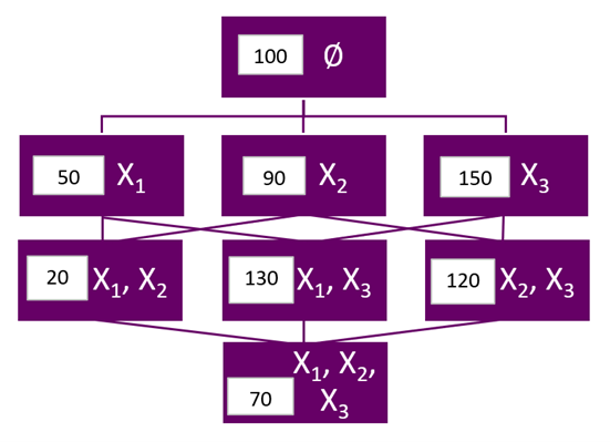
The top node represents the null model – a model containing no predictor variables and producing an overall prediction of 100. The next level of models represents one-variable models with respective predictions of 50, 90 and 150. Similarly, level three is occupied by two-variable models with respective predictions of 20, 130 and 120. Finally, the last node reflects the model being evaluated - with all three variables and a prediction of 70. The edges in the diagram connect models that differ by only one variable. For example, the final node and the middle node from the level above differ only by the X₂ variable.

To calculate the Shapley value of the variable X₂, the formula tells us that we need to aggregate the weighted marginal contributions of X₂ across all models that contain the variable X₂. Each marginal contribution is represented by the edge containing two successive models, where the lower-level model contains X₂, and the higher-level model does not. Each marginal contribution is weighted by its respective binomial coefficient, multiplied by the number of variables in the model being considered for the marginal contribution. After some simple math, the formulaic expression for the weights becomes

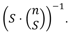
Stated differently, the weight of the marginal contribution of X₂ in a model with S predictor variables would be the reciprocal of the number of possible marginal contributions to models with S predictors, or equivalently the number of edges in the level of that model. This also means that the sum of the weights in any one level should equal the sum of the weights of any other level, and the total sum of all weights should equal one. For example, there are six possible contributions to all two-variable models, i.e., six edges in the level of the two-variable models, so the weight for any marginal contribution of this level in the diagram would be 1/6.

Using the numbers from the diagram, the marginal contribution of X₂ between the null model and the one-variable model is 90 - 100 = -10. Similarly, the marginal contribution of X₂ between the full model and the first, two-variable, model from the level above is 70 – 20 = 50. Aggregating all marginal contributions in this fashion, we get (1/3)*(90 - 100) + (1/6)* (20 - 50) + (1/6)* (120 - 150) + (1/3)*(70 - 130) = -33.  In other words, the overall effect of the variable X₂ in the full, three-variable, model is to reduce the average prediction of the null model by 33. Because this effect describes the variable contribution to the prediction for an individual data point, this type of model interpretation is called local.

As an exercise, you can try calculating the Shapley values of the other two predictors. When you add the Shapley values of all three predictors, you should get the difference between the prediction of the full model, 70, and the prediction of the null model, 100, which equals -30.

This simple example demonstrates how Shapley values can break down a model's output into individual contributions from each input feature. Unfortunately, Shapley values are not universal, and care must be exercised in how we apply and interpret their implementation. There are several important practical limitations that could result in misleading explanations. Shapley values can also be aggregated across all predictions to represent the global effect of a given feature. In a future blog post, I will explore these additional topics in more detail, so stay tuned!

References:

1. Shapley, Lloyd S. (August 21, 1951). "Notes on the n-Person Game -- II: The Value of an n-Person Game" (PDF). Santa Monica, Calif.: RAND Corporation.
2.  https://en.wikipedia.org/wiki/Shapley_value